Rolling shutter cameras

We want to find the absolute pose for a calibrated rolling shutter camera. Suppose we have the following information available:

• A set of 3D scene points expressed in the world coordinate frame.
• Sets of 2D points in the two-dimensional images, where each set corresponds to one 3D point.

Let us load the data:

using DelimitedFiles
link1 = "https://gist.githubusercontent.com/PBrdng/e17d0e3bc4d983734238b9cb8386d560/raw/07272b125a6ad03c791fdf99e741318f1d85149b/3Dpoints"
link2 = "https://gist.githubusercontent.com/PBrdng/e17d0e3bc4d983734238b9cb8386d560/raw/07272b125a6ad03c791fdf99e741318f1d85149b/2Dpoints"
points3D = readdlm(download(link1)) |> transpose
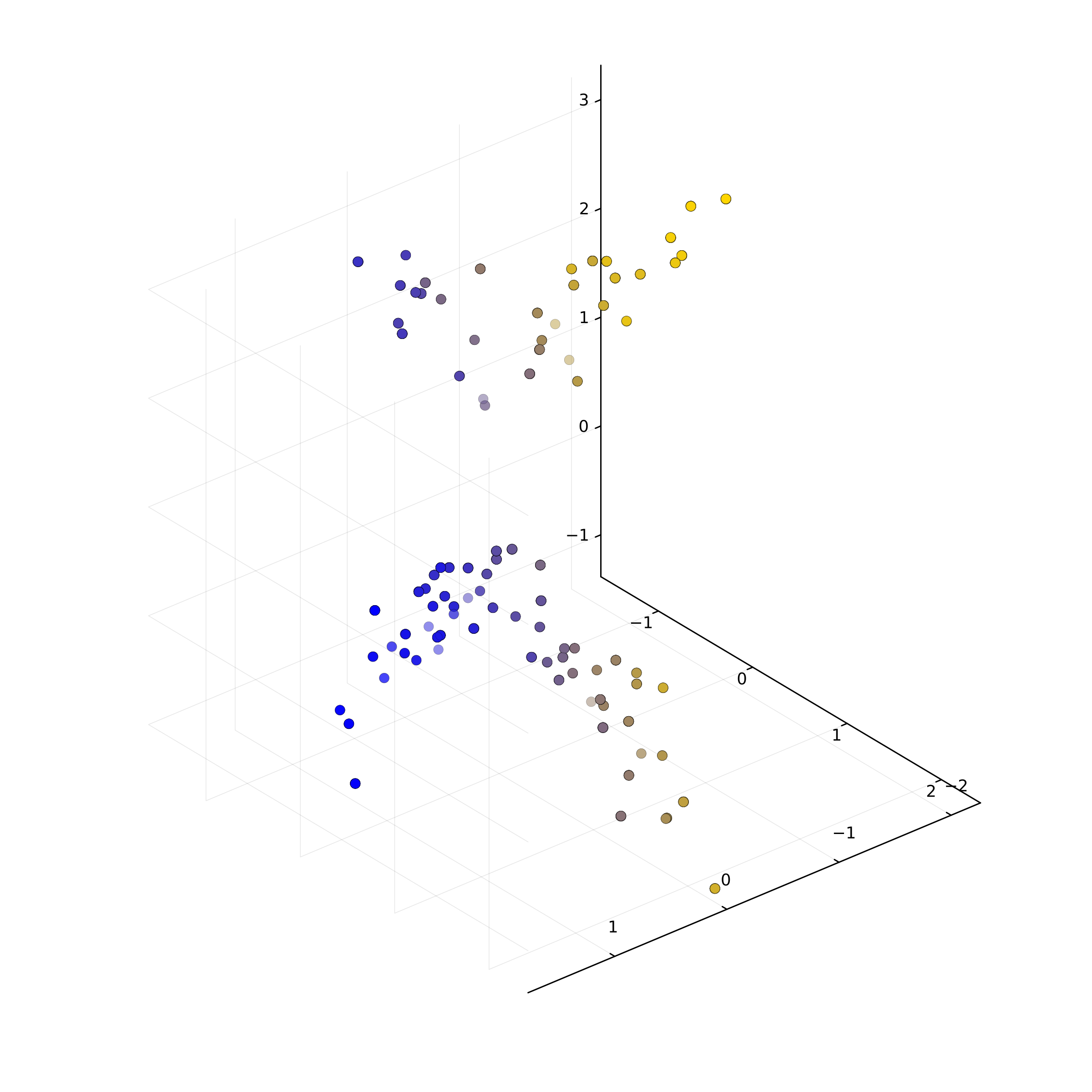
points2D = readdlm(download(link2)) |> transpose

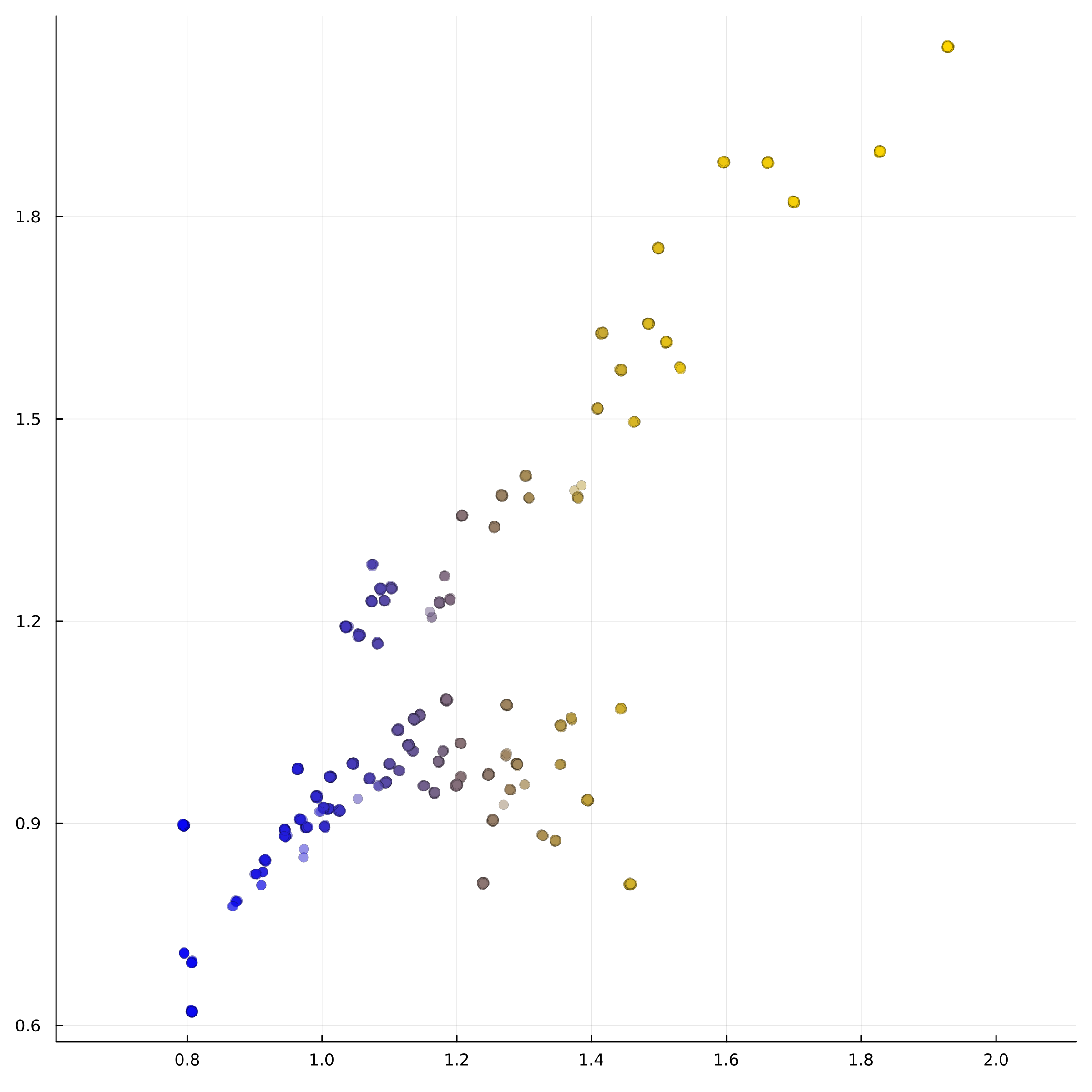
Now points2D is a $3\times N$ matrix, where $N$ is the number of images. The first two rows of points2D are the coordinates of the respective images, and the third row gives the scanlines. A rolling shutter camera captures images line by line over time. These lines are called scanlines.

Similarly points3D is a $4\times N$ matrix, where $N$ is the number of images. The columns of points2D and points3D are synchronized in the sense that the $i$-th column of points2D is the image of the $i$-th column of points3D.

We want to reconstruct the camera from this data. For this, we use a model introduced by Saurer et al.¹. Their morel introduces a linear velocity in the camera projection matrix to approximate the motion of the rolling shutter camera. Furthermore, the model assumes that each scanline takes exactly the same time, and the relative camera translation $t_n$ at the $n$-th scanline is

$$ t_n = \mathbf{v}n \tau \quad $$

where $\mathbf{v}\in\mathbb R^3$ denotes the constant linear camera velocity, and $\tau$ is the time taken to complete each scanline, and $n$ ist the number of scanline. Making the assumption of a constant linear velocity, we can express a pixel on the $n$th scanline as:

$$x_n = \begin{bmatrix} R & t - t_n \end{bmatrix} X,$$

where $R$ is an orthogonal matrix (we assume calibrated cameras).

The variables $R$ and $t$ describe the camera’s position and orientation in the world frame, which is also its position for the first captured scanline. The variable $t_n$ represents the camera’s position for the $n$-th scanline. The correspondence between $x_n$ and $X$ signifies a relationship between a 2D point in the image and its corresponding 3D point. The given data in this equation consist of a set of 2D image points denoted by $x_n$ and their corresponding 3D points represented by $X$. The unknowns in this equation are $R$, $t$, and the linear velocity $v$ in $t_n$, amounting to a total of 9 degrees of freedom (3 each for $R$, $t$, and $v$). Consequently, we need at least

$$ m = 5$$

images for reconstruction.

By taking the cross product of $x_n$ , we obtain $x_n \times (\begin{bmatrix} R & t - t_n \end{bmatrix} X) = 0$ Assuming noisy data, we attempt to reconstruct $R,t$ and $v$ by solving the optimization problem

$$\min\quad \left\Vert x_n \times (\begin{bmatrix} R & t - t_n \end{bmatrix} X)\right\Vert. $$

Implementation with Homotopy Continuation

Now let's solve this optimization problem using homotopy continuation by solving the critical equations. In our case we have

$$\tau = 0.01.$$

using HomotopyContinuation, LinearAlgebra, StatsBase

τ = 0.01
m = 5
@var x[1:3, 1:m], u[1:2, 1:m]
@var R[1:3, 1:3], t[1:3], v[1:3], n[1:m]

cams = [[R t-(n[i]*τ).*v] for i in 1:m] # m = 5 cameras

y = [cams[i] * [x[:,i]; 1] for i in 1:m] # m = 5 images

Now we define the function that we want to minimize.

g = [cross(y[i],  [u[:,i]; 1]) for i in 1:m]

Since $R$ is constrained to be an orthogonal matrix and $v$ is constrained to have norm $1$, we use Lagrange multipliers for optimization.

k = R * R' - diagm(ones(3))
Rconstraints = [k[i,j] for i in 1:3, j in 1:3 if i<=j]
vconstraints = transpose(v) * v - 1

@var l1[1:6], l2       # Lagrange multipliers 

L = transpose(g) * g - transpose(l1) * Rconstraints - l2 * vconstraints
Lag = differentiate(L, [vec(R); t; v; l1; l2]);

F = System(Lag, variables = [vec(R); t; v; l1; l2], parameters = [vec(x); vec([u; n'])]);

Solving F then gives all critical points. We want to solve this system many times for different parameters.
First, we need an initial solution for a random set of parameters.

p0 = randn(ComplexF64, 30) 
S0 = solve(F, target_parameters = p0)
start = solutions(S0);

The array start contains 480 solutions. Now, we track these 80 solutions towards the photo parameters we are interested in

N = size(points2D, 2)
s = StatsBase.sample(collect(1:N), m; replace=false)

X = points2D[1:3, s] 
Y = points2D[:, s]

p1 = [vec(X); vec(Y)]
S1 = solve(F, start, start_parameters = p0, target_parameters = p1) 

We solved the system F using parameter homotopies, with the start parameter p0 and the target parameter p1.
Then we evaluate each solution r with the parameter r computing the norm of g(r,p) and return the solution that has the smallest norm.

G = System(vcat(g...), variables = [vec(R); t; v], parameters = [vec(x); vec([u; n'])]);
function find_min(sols, p)
    sols = [r[1:15] for r in sols]
    a = map(sols) do r 
        norm(G(r, p))
    end
    i = findmin(a)
    sols[i[2]]
end
recovery = find_min(real_solutions(S1), p1)
R1, t1, v1 = reshape(recovery[1:9], 3, 3), recovery[10:12], recovery[13:15]

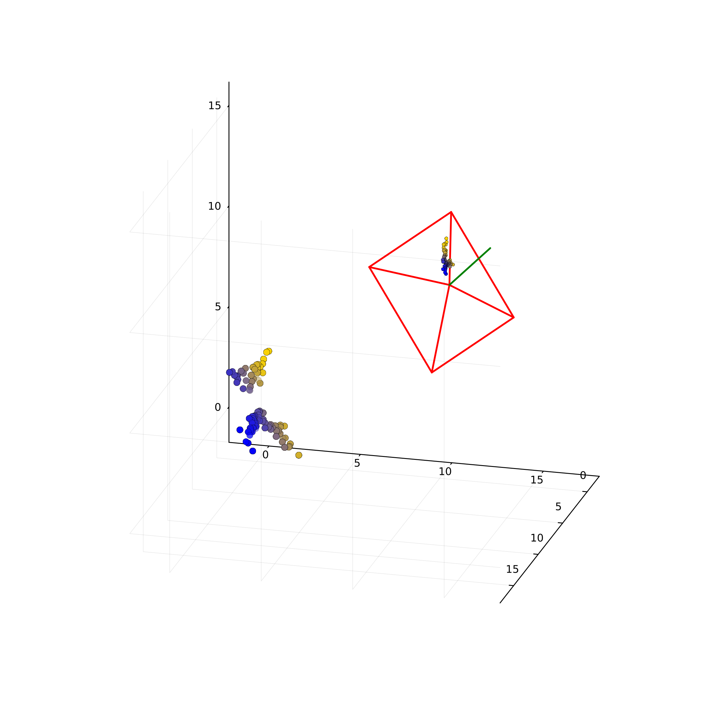
Here is the reconstructed data:

Published by Rami Abuzerr, Paul Breiding 26 Mar, 2019